This site presents the products of BESA GmbH, the leading innovators in digital EEG and MEG software for research and clinical applications.
- BESA Research 7.1 January 2024 is released!
Download the latest BESA Research version here!
Features in BESA Connectivity 2.0
NOTE that BESA Connectivity 2.0 is for research use only!
Many exciting features are available in BESA Connectivity 2.0. A non-exhaustive overview:
General
- Optimized, user-guided workflows for time-frequency and connectivity analysis of EEG/MEG data
- All analyses are computed automatically; user interaction steps required are reduced to a minimum
- The time-frequency and connectivity values computed in BESA Connectivity can be directly used for scientific reports
- The outcomes can be exported in open ASCII formats for further statistical analysis
- All results are visualized and can be directly used for publications
- BESA Connectivity 2.0 integrates optimally with data that were analyzed in BESA Research 7.0 or higher, but it can also process data from other software packages as long as they conform to the BESA Connectivity file format
- Input data can be provided in sensor space (surface EEG/MEG channels, or polygraphic channels), or in source space (virtual channels located inside the brain, e.g. from a source montage)
- Batch processing of multiple subjects is supported
- Grand average calculations and displays
- Several colour maps are available, and two themes are supported: BESA White and BESA Standard
Batch processing of several subjects in one go
Time-Frequency Analysis
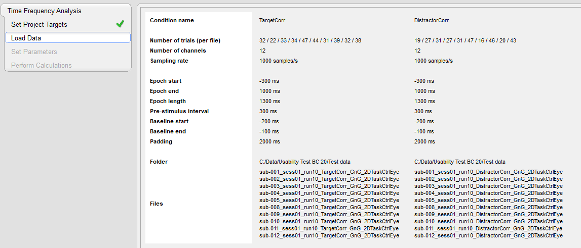
- BESA Connectivity 2.0 offers a batch processing mode in time-frequency projects that allows loading data sets for multiple subjects simultaneously and processes all those data sets in one project. Up to 10 different conditions are supported. For each condition, it is possible to select several data sets in the Load Data dialog (see figure above).
- Grand Average views and data exports of multi-subject time-frequency analysis are available.
- In BESA Connectivity 2.0, three approaches for computing time-frequency decomposition are provided:
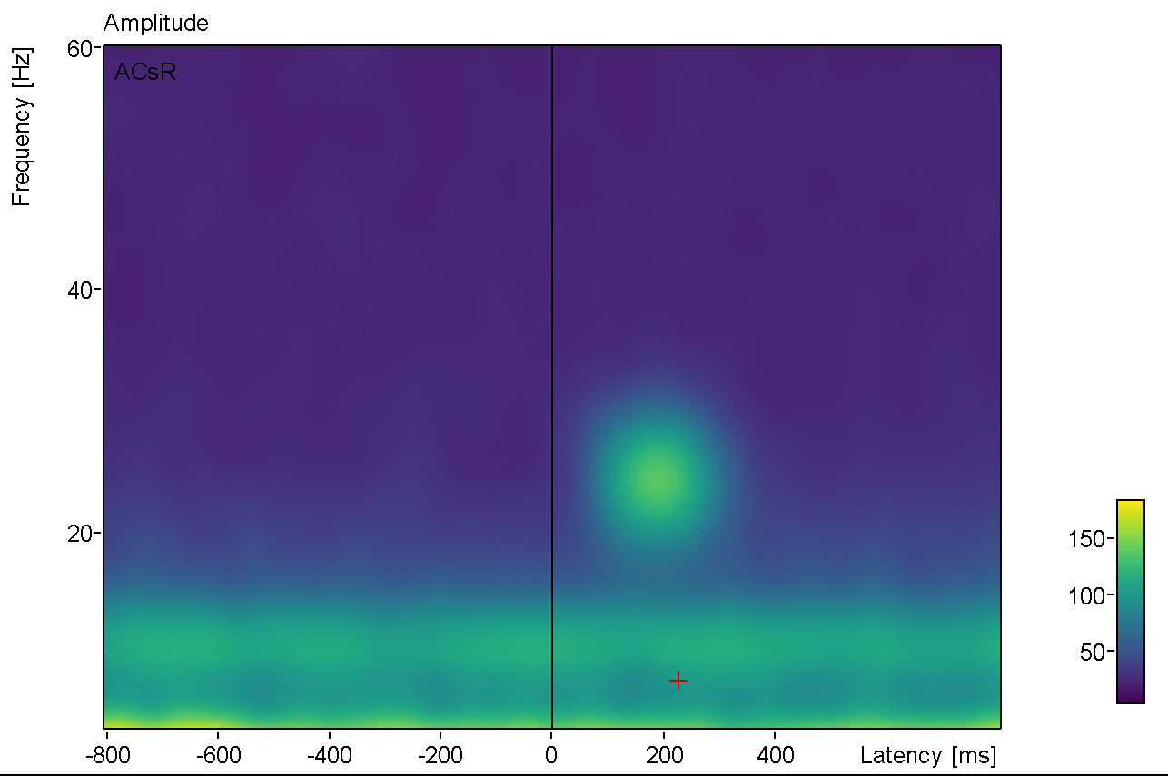
- Complex Demodulation is based on the convolution of the EEG/MEG signal with series of sine and cosine waves.
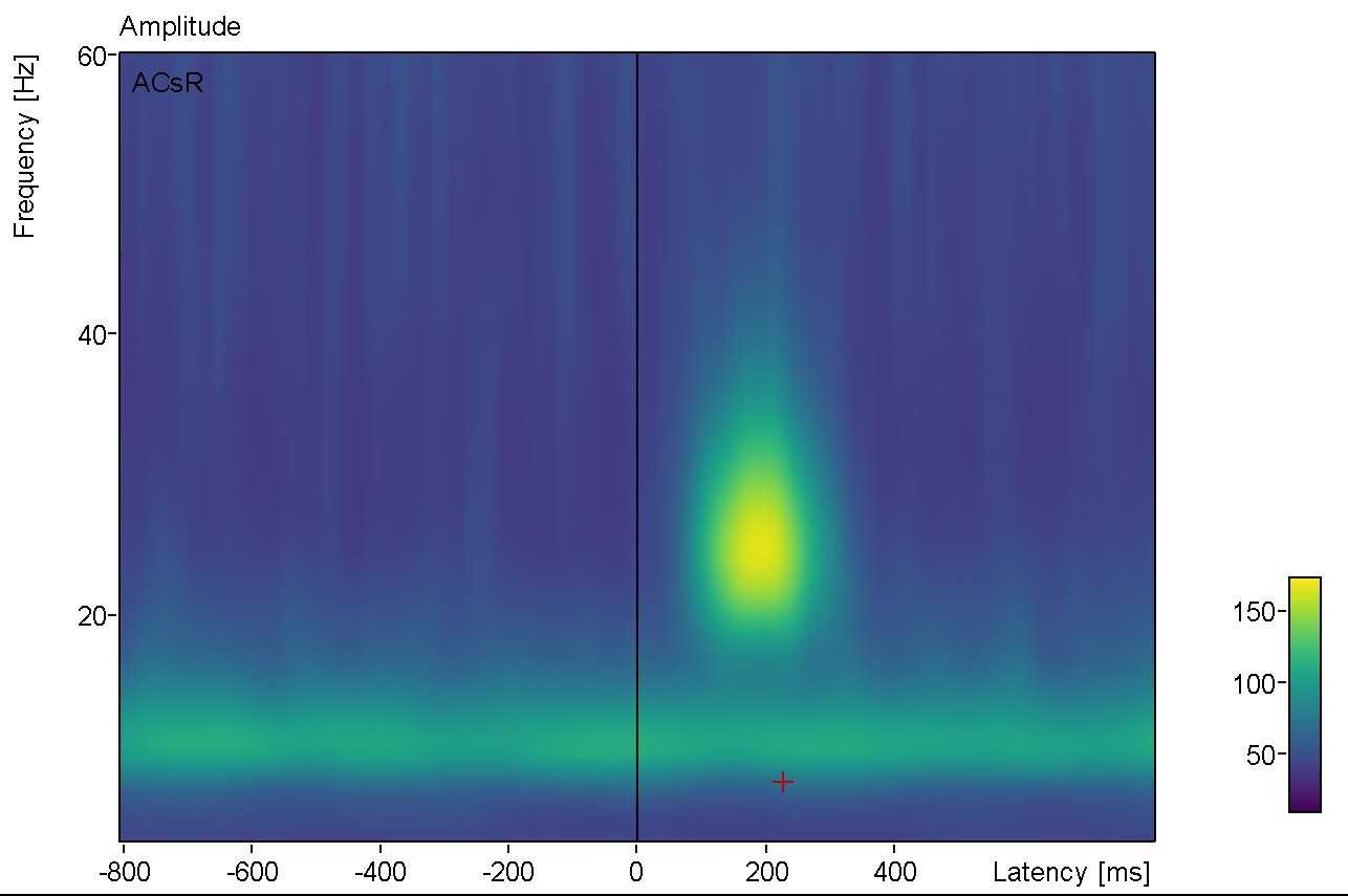
- Wavelet Transform uses series of complex Morlet wavelets or Mexican Hat wavelets to extract the magnitude and phase information.
- A multi-taper method is introduced to the time-frequency methods. Multitaper analysis uses several tapers to decompose the signal into its frequencies. Here, Slepian Sequences are used to construct the tapers, which are then used in a time-frequency decomposition of the signal. Multitapering combines the properties of the different tapers to control the leakage and smooth the signal in the frequency domain. The multitaper transformation uses a sliding time window with a length that decreases with increasing frequency.
- Data export:
- Export project results: Averaged time-frequency results of all decompositions and data sets are exported. They can directly be read in to BESA Statistics.
- Averaged TF data: Selected display type options (temporal-spectral evolution (TSE) or absolute (ABS) values for amplitude or power) are considered during export.
| Complex demodulation | Wavelet | Multitaper |
|---|---|---|
 |
 |
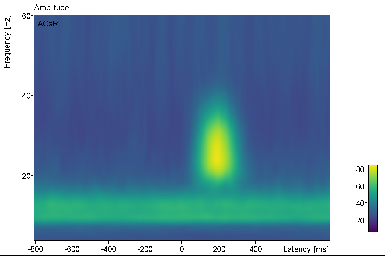 |
| CD offers a constant time-frequency resolution | Wavelet optimizes time-frequency resolution | Multitaper creates smooth signal at higher frequencies |
Connectivity Analysis
- Batch processing: When loading a time-frequency project containing multiple conditions with multiple data files, connectivity analysis for all those data files can be computed within one project.
- Grand Average views and data exports of multi-subject connectivity analysis are available.
- Nine connectivity methods:
- Phase-based methods:
- Coherence
- Imaginary Part of Coherency
- Phase Locking Value
- Phase lag index (PLI) (Stam et al. 2007)
- Weighted phase lag index (WPLI) (Vinck et al., 2011)
- Directed phase lag index (dPLI) (Stam and van Straaten, 2012)
- Granger Causality-based methods:
- Granger Causality
- Partial Directed Coherence
- Directed Transfer Function
- Phase-based methods:
- TFC grid view to show all connectivities in one view
- 3D view to show connectivities in the brain / on the scalp surface
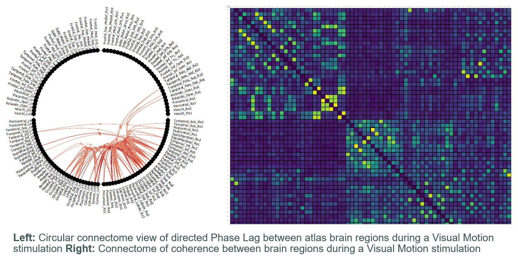
- Circular Graph View: This visualization mode places the sources (or sensors) on a circle and shows the coupling strength as connections for the selected latency & frequency bin between all combinations of sources. The channels are automatically arranged in four quadrants (left anterior / right anterior / left posterior / right posterior) to facilitate interpretation.
- Simultaneous averaging over time and frequency: when both averaging options are selected the matrix view changes to a visualization of a single tile per connection, thus enabling a connectome view for the selected time-frequency range.
- Freeze-Pane mode for TFC View: Channel labels will remain visible at the left-most column and top-most row of the matrix display even if the visualization is zoomed by the user.
- The 3D visualization takes into account the colors and sizes of the sources specified in the BESA Solution File Format (*.bsa).
- Data export:
- Export project results: Connectivity results of all selected methods and data sets are exported. They can directly be read in to BESA Statistics.
Recent Comments