- Neurosciences

NIRx
High-resolution portable and
desktop fNIRS systems
NordicNeuroLab
Solution for functional MRI
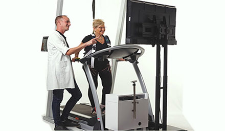
Ergospect
Innovative Ergometers for MR Imaging
Dixi
Intracerebral Electrodes for
localization of epileptic foci
Persyst
EEG Review and
Analysis Software
Suricog
Innovative Eye Powered Interactivity
Brain Products
Solutions for
Neurophysiology Research
CGX
Wireless EEG
Headset
Medoc
Quantitative Sensory
Testing (QST) devices
PST
Research devices for
experiment design
BESA
Software for EEG and
MEG research
Magventure
Transcranial Magnetic Stimulators
Soterix
Transcranial Direct
Current Stimulators
Localite
Navigator for TMS Coil & EEG Electrode placement
Axilium
Robotic Navigation
for TMS Coils.
Storz - Neurolith
Extracorporeal shock wave therapy - Sports & Rehabilitation
Storz - ESWT
Extracorporeal
shock wave therapy
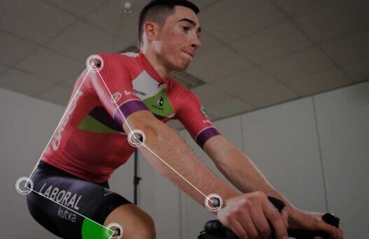
Noraxon
EMG and IMU Based
Motion Tracking
Lojer
Most versatile
treatment table
U & O
UAN.GO -
innovative exoskeleton
Codamotion
Digital Infrared based
motion tracking
Euleria
Measurable rehabilitation
Roceso
Robotic and Digital Health Solutions
Kinestica
Advanced Neurological Rehabilitation
Mectronic
High-Performance Therapies
GaitBetter
Gait Rehabilitation
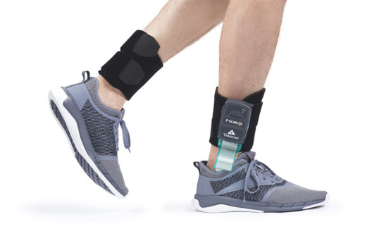
Tekscan
Force Measurement
STT
Inertial Motion Analysis
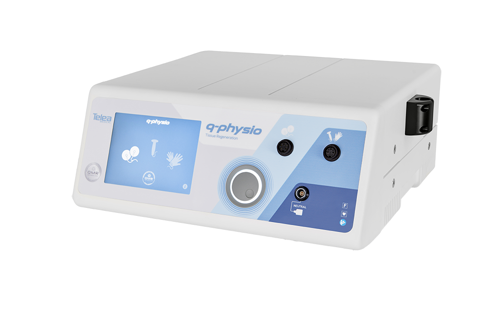
Telea Medical
QMR Therapy - Vascular
Atys Medical
Peripheral vascular testing systems
Medis
Patient Monitoring & Cardio-vascular Diagnosis - Asthetics
Storz - ESWT
Extracorporeal
shock wave therapy