Blood tests could soon predict your risk of Alzheimer’s
Many Alzheimer’s researchers, neurologist Randall Bateman is not prone to effusiveness, having endured disappointments in his field. But he and others have found one big


Many Alzheimer’s researchers, neurologist Randall Bateman is not prone to effusiveness, having endured disappointments in his field. But he and others have found one big
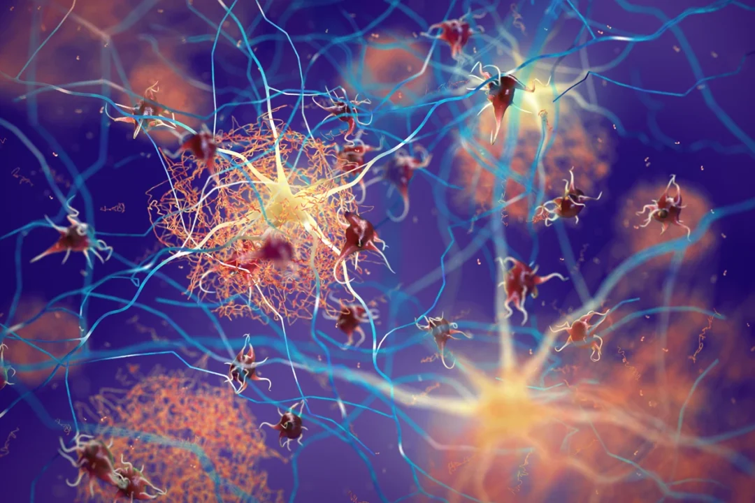
Alzheimer’s disease is a brain disorder that causes problems with memory, mood, and the ability to perform daily activities. Although there are medicines available to
Alzheimer’s disease (AD) is a neurodegenerative disorder that dramatically affects cognitive abilities and represents the most common cause of dementia.

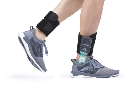
For orthopaedic specialists Dr Rudolf Lassel and Dr Suchung Kim from Berlin, Extracorporeal Shock Wave Therapy (ESWT) is a fundamental component of their everyday work – particularly
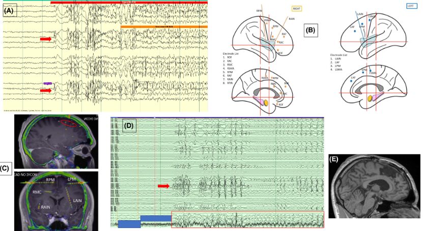
Epilepsy surgery is the therapy of choice for many patients with drug-resistantfocal epilepsy. Recognizing and describing ictal and interictal patterns with in-tracranial electroencephalography (EEG) recordings
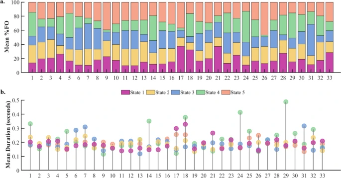
Task-free brain activity exhibits spontaneous fluctuations between functional states, characterized by synchronized activation patterns in distributed resting-state (RS) brain networks.
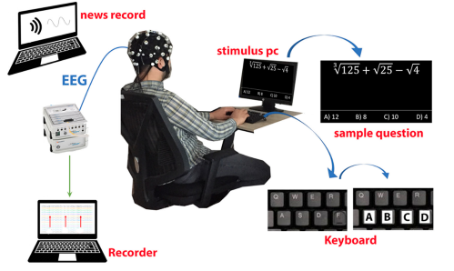
Cognitive fatigue occurs in various situations and is an essential condition to detect. In this study, how single and multi-tasking tests affect cognitive workload was

Inhibitory control has been linked to beta oscillations in the fronto-basal ganglia network. Here we aim to investigate the functional role of the phase of
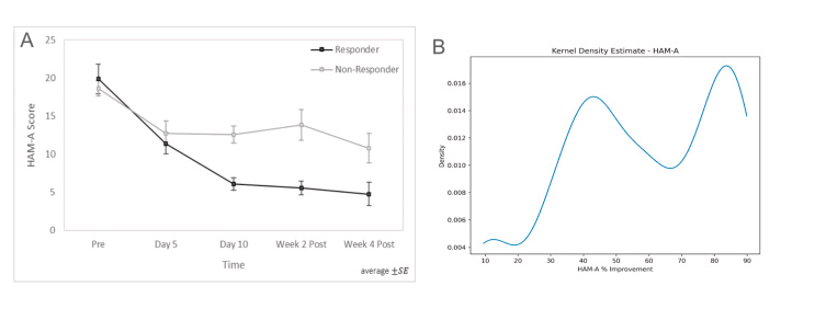
Generalized anxiety disorder (GAD) is one of the most common conditions affecting adolescents and young adults, with prevalence increasing markedly over the past decade
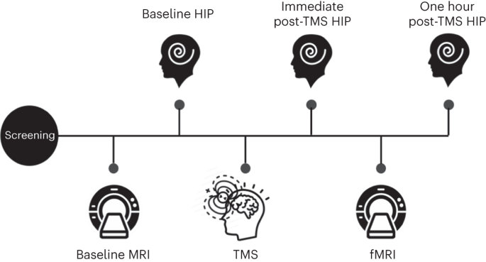
Hypnotizability, one’s ability to experience cognitive, emotional, behavioral and physical changes in response to suggestions in the context of hypnosis, is a stable neurobehavioral trait