
Do all dogs feel pain the same? Quantitative Sensory Testing in Man’s Best Friend
Pain sensitivity in dogs – It may not be what you thought (It definitely wasn’t what we thought with our old friend, Mutchie)


Pain sensitivity in dogs – It may not be what you thought (It definitely wasn’t what we thought with our old friend, Mutchie)
6.1 million patients suffer from Parkinson’s Disease (PD) in the world today. A progressive neurogenerative disease, that is both chronic and complex, PD’s etiology is
In order to test the hyperscanning capability of the X.on, we took 10 headsets, paired each of them with an Android™ phone, and set all
Emotions are an important part of our lives, and understanding how they emerge holds great relevance not only for basic neuroscience but also for clinical
More and more researchers all over the world are using Lab Streaming Layer (LSL) and we at Brain Products continue to put focus on this
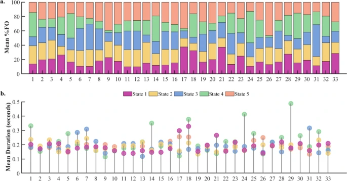
Task-free brain activity exhibits spontaneous fluctuations between functional states, characterized by synchronized activation patterns in distributed resting-state (RS) brain networks.
Sickle cell disease (SCD) is a genetic disorder causing painful and unpredictable Vaso-occlusive crises (VOCs) through blood vessel blockages
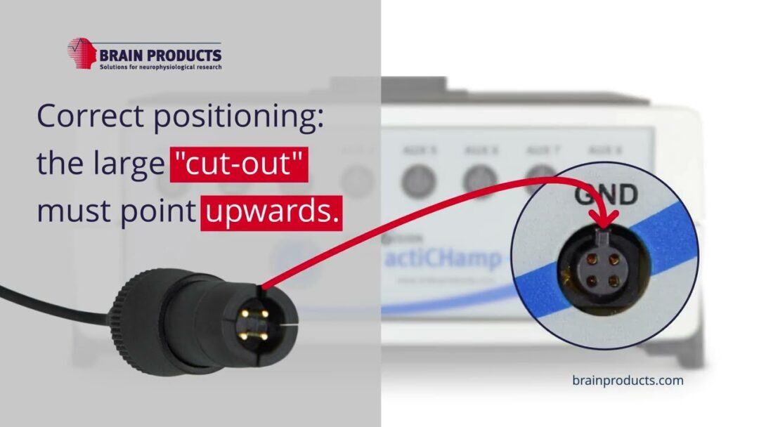
This tutorial video demonstrates how to connect the ground electrode properly to the actiCHamp Plus amplifier.
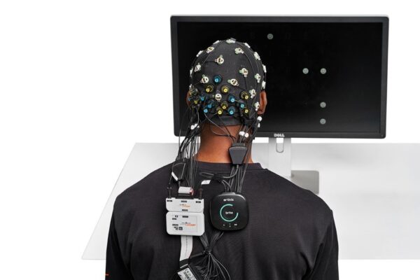
In this article, you will find resources specific to the combination of the LiveAmp with actiCAP slim electrodes and Artinis Brite fNIRS. The information covered here, should be used together with the
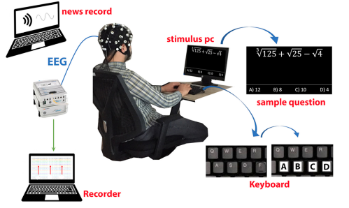
Cognitive fatigue occurs in various situations and is an essential condition to detect. In this study, how single and multi-tasking tests affect cognitive workload was